Ray Casting

This page describes the mathematical theory behind the ray casting algorithms implemented in Crater.rs. Ray casting has been fundamental to computer graphics since the early work of Appel 6.

Mathematical Foundation

Ray casting is the computational problem of finding a tensor ${\Lambda }^i$ such that $F^i(S^{ij}({\Lambda }^i))=0^i$, where $S^{ij}$ is the function representing ray extensions:

$$S^{ij}({\Lambda }^i)=X^{ij}+{\Lambda }^i{U}^{ij}$$

Here, $X^{ij}$ represents ray origins and $U^{ij}$ represents ray directions.

This library implements multiple algorithms for determining ray intersections with isosurfaces and regions. The algorithms are configured via the RayCastAlgorithm enum.

Analytical Method

The analytical method for computing ray intersections is a special, but highly performant and precise algorithm. This algorithm computes the intersection point analytically, by making the above 1-D implicit function explicit:

$$F^i(S^{ij}({\Lambda }^i))=0^i$$

is reformulated as:

$${\Lambda }^i=R^i(X^{ij},U^{ij})$$

Where $R^i$ is a RayField. RayFields are similar to ScalarFields, but take an extra input parameter, a tensor of unit directions $U^{ij}$. The field returns the rank-1 tensor of distances from $X^{ij}$ to the point at which $F^i(S^{ij}({\Lambda }^i))=0^i$ along the direction $U^{ij}$.

A valid $R^i$ may not be analytically available. Therefore, the analytical method is not available generally, for all $F^i$. For common ScalarFields in this library, the mapping $F^i\to R^i$ is implemented already.

Concrete Implementations

(Hyper)planes

For a hyperplane with normal vector $n^j$, we define the following two quantities:

$${\alpha }^i=X^{ij}{n}_j$$ $${\beta }^i=U^{ij}{n}_j$$

Then, the ray field is:

$$R^i(X^{ij},U^{ij})=\frac{{\alpha }^i}{{\beta }^i}$$

There are a few degenerate cases:

• If ${\beta }^i=0$, then the ray is parallel to the hyperplane, and the ray field is undefined.
• If ${\alpha }^i=0$, then the ray origin is on the hyperplane.
• If $\frac{{\alpha }^i}{{\beta }^i}<0$, then the ray intersection is behind the ray origin.

(Hyper)spheres

For a hypersphere with radius $r$, the primal scalar field is defined as:

$$F^i(X^{ij})=X^{ij}{X}_j^i-r^2$$

For ray intersections, the 1-D implicit function is:

$$\begin{array}{rl}{0}^i& =F^i(X^{ij}+{\Lambda }^i{U}^{ij})\\ & =(X^{ij}+{\Lambda }^i{U}^{ij})(X_j^i+{\Lambda }^i{U}_j^i)-r^2\\ & =X^{ij}{X}_j^i+{\Lambda }^i{X}^{ij}{U}_j^i+{\Lambda }^i{U}^{ij}{X}_j^i+{\Lambda }^i{\Lambda }^i{U}^{ij}{U}_j^i-r^2\\ & =X^{ij}{X}_j^i+2{\Lambda }^i{X}^{ij}{U}_j^i+{\Lambda }^i{\Lambda }_i{U}^{ij}{U}_j^i-r^2\\ & =(U^{ij}{U}_j^i){\Lambda }^i{\Lambda }^i+(2X^{ij}{U}_j^i){\Lambda }^i+(X^{ij}{X}_j^i-r^2)\end{array}$$

The final equation is a quadratic form over ${\Lambda }^i$. Using the quadratic equation:

$$\begin{array}{rl}{a}^i& =U^{ij}{U}_j^i\\ b^i& =2X^{ij}{U}_j^i\\ c^i& =X^{ij}{X}_j^i-r^2\end{array}$$

The discriminant is:

$${\Delta }^i=b^i{b}_i-4a^i{c}^i$$

The possible solutions for ${\Lambda }^i$ take the form:

$${\Lambda }^i=\frac{-b^i\pm \sqrt{b^i{b}^i-4a^i{c}^i}}{2a^i}$$

There are a few cases:

• If ${\Delta }^i<0$, then the ray does not intersect the sphere.
• If ${\Delta }^i=0$, then the ray intersects the sphere at a single point (tangent).
• If ${\Delta }^i>0$, then the ray intersects the sphere at two points, one or both of which may be behind the ray.

In all cases, we take the smallest non-negative root.

(Hyper)cones

The primal scalar field for a cone with unit-axis $a^j$ and opening angle $\theta$ is defined as:

$$F^i(X^{ij})=(X^{ij}{a}_j{)}^2-\cos (\theta {)}^2(X^{ij}{X}_j^i)$$

For ray intersections, the 1-D implicit function is:

$$\begin{array}{rl}{0}^i& =F^i(X^{ij}+{\Lambda }^i{U}^{ij})\\ & =((X^{ij}+{\Lambda }^i{U}^{ij})a_j{)}^2-\cos (\theta {)}^2((X^{ij}+{\Lambda }^i{U}^{ij})(X_j^i+{\Lambda }^i{U}_j^i))\\ & =(X^{ij}{a}_j+{\Lambda }^i{U}^{ij}{a}_j{)}^2-\cos (\theta {)}^2(X^{ij}{X}_j^i+{\Lambda }^i{X}^{ij}{U}_j^i+{\Lambda }^i{U}^{ij}{X}_j^i+{\Lambda }^i{\Lambda }^i{U}^{ij}{U}_j^i)\\ & =(X^{ij}{a}_j{)}^2+2{\Lambda }^i{X}^{ij}{a}_j{U}_j^i+{\Lambda }^i{\Lambda }^i(U^{ij}{a}_j{)}^2-\cos (\theta {)}^2(X^{ij}{X}_j^i+2{\Lambda }^i{X}^{ij}{U}_j^i+{\Lambda }^i{\Lambda }^i{U}^{ij}{U}_j^i)\\ & =((U^{ij}{a}_j{)}^2-\cos (\theta {)}^2{U}^{ij}{U}_j^i){\Lambda }^i{\Lambda }^i+(2X^{ij}{U}_j^i)(a_j-\cos (\theta {)}^2){\Lambda }^i+(X^{ij}{a}_j{)}^2-\cos (\theta {)}^2(X^{ij}{X}_j^i)\end{array}$$

The final equation is a quadratic form over ${\Lambda }^i$. Using the quadratic equation:

$$\begin{array}{rl}{a}^i& =(U^{ij}{a}_j{)}^2-\cos (\theta {)}^2{U}^{ij}{U}_j^i\\ b^i& =2X^{ij}{U}_j^i(a_j-\cos (\theta {)}^2)\\ c^i& =(X^{ij}{a}_j{)}^2-\cos (\theta {)}^2(X^{ij}{X}_j^i)\end{array}$$

The discriminant is:

$${\Delta }^i=b^i{b}^i-4a^i{c}^i$$

The possible solutions for ${\Lambda }^i$ take the form:

$${\Lambda }^i=\frac{-b^i\pm \sqrt{b^i{b}^i-4a^i{c}^i}}{2a^i}$$

There are a few cases:

• If ${\Delta }^i<0$, then the ray does not intersect the cone.
• If ${\Delta }^i=0$, then the ray intersects the cone at a single point (tangent).
• If ${\Delta }^i>0$, then the ray intersects the cone at two points, one or both of which may be behind the ray.

In all cases, we take the smallest non-negative root.

(Hyper)cylinders

The primal scalar field for a hypercylinder with radius $r$ extending along the last dimension is defined as:

$$F^i(X^{ij})=\sum _{k=1}^{N-1}(X^{ik}{)}^2-r^2$$

where the summation is over the first $N-1$ dimensions. For ray intersections, we project the problem to the first $N-1$ dimensions:

Let $X^{\prime i(N-1)}=X^{ij}$ for $j\in [1,N-1]$ and $U^{\prime i(N-1)}=U^{ij}$ for $j\in [1,N-1]$.

The 1-D implicit function becomes:

$$\begin{array}{rl}{0}^i& =F^i(X^{\prime i(N-1)}+{\Lambda }^i{U}^{\prime i(N-1)})\\ & =(X^{\prime i(N-1)}+{\Lambda }^i{U}^{\prime i(N-1)})(X_{(N-1)}^{\prime i}+{\Lambda }^i{U}_{(N-1)}^{\prime i})-r^2\\ & =X^{\prime i(N-1)}{X}_{(N-1)}^{\prime i}+2{\Lambda }^i{X}^{\prime i(N-1)}{U}_{(N-1)}^{\prime i}+{\Lambda }^i{\Lambda }^i{U}^{\prime i(N-1)}{U}_{(N-1)}^{\prime i}-r^2\end{array}$$

This reduces to a quadratic form with coefficients:

$$\begin{array}{rl}{a}^i& =U^{\prime i(N-1)}{U}_{(N-1)}^{\prime i}\\ b^i& =2X^{\prime i(N-1)}{U}_{(N-1)}^{\prime i}\\ c^i& =X^{\prime i(N-1)}{X}_{(N-1)}^{\prime i}-r^2\end{array}$$

The solutions follow the same quadratic formula as hyperspheres, taking the smallest non-negative root.

(Hyper)tori

The primal scalar field for a hypertorus with major radius $r_1$ and minor radius $r_2$ is defined as:

$$F^i(X^{ij})={\left(\sqrt{\sum _{k=1}^{N-1}(X^{ik}{)}^2}-r_1\right)}^2+(X^{iN}{)}^2-r_2^2$$

For ray intersections, the analytical solution involves solving a quartic equation, which is significantly more complex than quadratic equations. Due to this complexity and numerical stability concerns, analytical solutions are not implemented for hypertori. Alternative approaches like sphere tracing 8 may be more suitable for such complex implicit surfaces.

Bracket and Bisect Algorithm

The ray casting process consists of two main steps:

1. Ray Bracketing: Finding intervals along rays that contain potential intersections
2. Ray Bisection: Refining these intervals to precisely locate intersection points

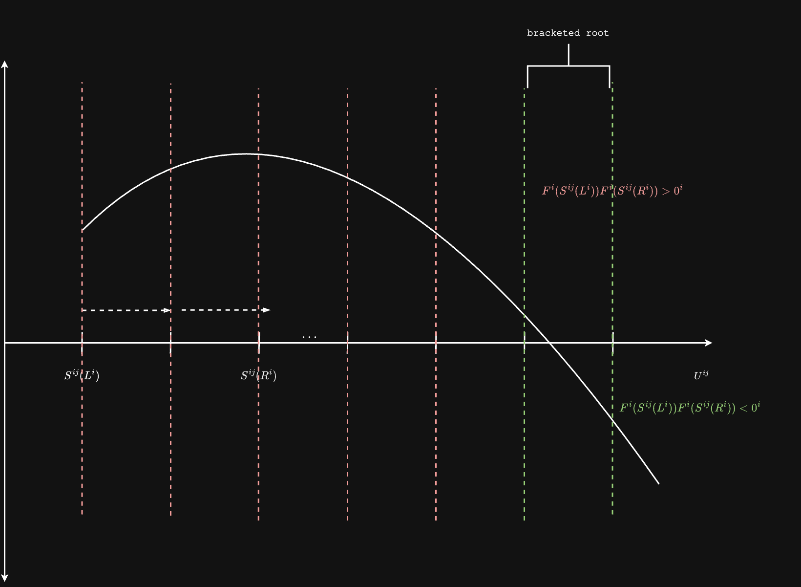
Ray Bracketing Algorithm

The ray bracketing algorithm efficiently finds intervals along rays that contain isosurface intersections. This implementation leverages tensor operations for parallel processing of multiple rays.

Algorithm Steps:

1. Initialize parameters:
   • Tensor field $F^i$, ray origins $X^{ij}$, unit directions $U^{ij}$
   • Step size $\Delta \lambda$, maximum iterations $K_{max}$
2. Initialize ray parameters:
   • $L^i\leftarrow 0$ (left bracket)
   • $R^i\leftarrow L^i$ (right bracket)
3. Iterate until convergence or max iterations:
   • Set $R^i\leftarrow L^i+\Delta \lambda$
   • Evaluate field at right bracket: $F^i(R^i)\leftarrow F^i(S^{ij}(R^i))$
   • Create mask for rays that don't yet have a bracket: $M^i\leftarrow {\mathbb{I}}^i\{F^i(S^{ij}(L^i))\cdot F^i(S^{ij}(R^i))\ge 0^i\}$
   • Update brackets using the mask
4. Return brackets $L^i,R^i$ such that $F^i(S^{ij}(L^i))\cdot F^i(S^{ij}(R^i))<0^i$

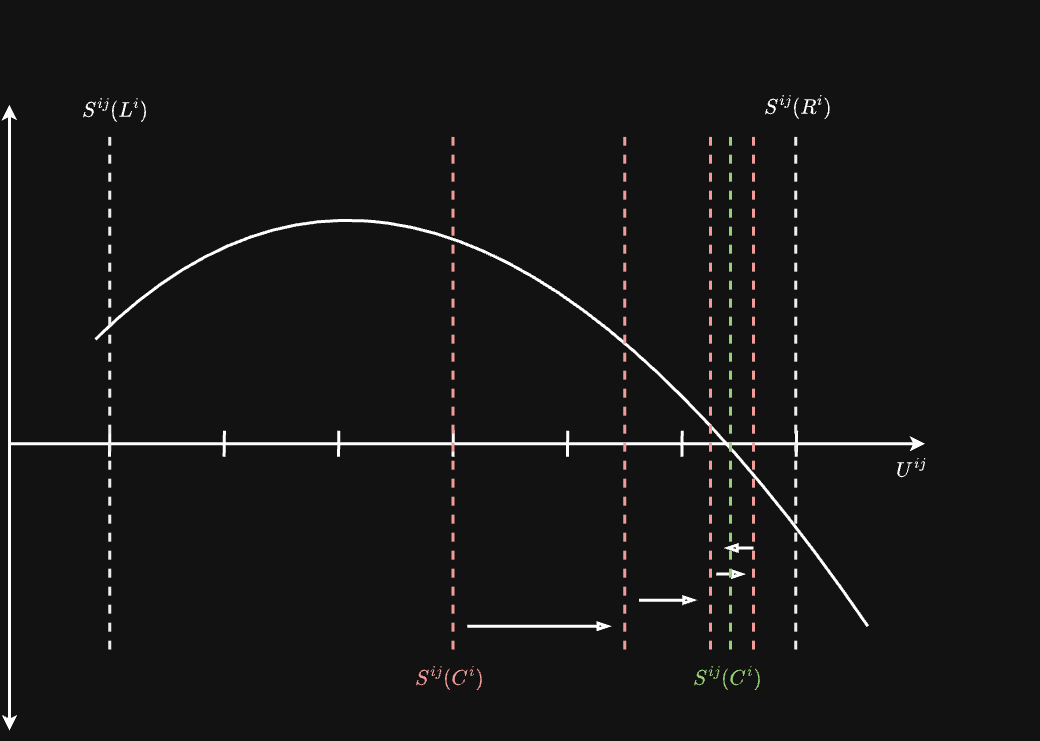
Ray Bisection Algorithm

After bracketing finds intervals containing isosurface intersections, the bisection algorithm refines these brackets to precisely locate the intersection points.

Algorithm Steps:

1. Initialize with bracketing tensors $L^i,R^i$ containing the isosurface
2. Iterate until convergence or max iterations:
   • Compute midpoint: $C^i\leftarrow (L^i+R^i)/2$
   • Create masks for which half contains the root:
     • ${\alpha }^i\leftarrow {\mathbb{I}}^i\{F^i(S^{ij}(L^i))\cdot F^i(S^{ij}(C^i))\ge 0^i\}$
     • ${\beta }^i\leftarrow {\mathbb{I}}^i\{F^i(S^{ij}(R^i))\cdot F^i(S^{ij}(C^i))\ge 0^i\}$
   • Update brackets based on which half contains the root
3. Return refined intersection points