Crater.rs: N-Dimensional Constructive Solid Geometry

crater.rs is a library for constructing and analyzing N-dimensional scalar fields. Primary features include:

• Constructive Solid Geometry (CSG) for N-dimensional scalar fields
• Ray casting for N-dimensional CSG regions
• Volume estimation for N-dimensional CSG regions
• Surface analysis for N-dimensional CSG regions
• Marching cubes for isosurface extraction
• Field visualization for N-dimensional scalar fields

Ready to start building? Head to Getting Started for installation instructions and your first example.

If you're not yet convinced, check out the Ray Casting Gallery, showing crater.rs's most sophisticated feature. This gallery is generated from the examples/raycast/gallery.rs example.

Citation and References

When using crater.rs in academic work, please cite:

@software{crater_rs,
  title={`crater.rs`: N-Dimensional Constructive Solid Geometry Library},
  author={Clyde Huibregtse},
  year={2025},
  url={https://gitlab.com/games1122013/crater.rs/},
  version={0.8.0}
}

Getting Started

This guide introduces you to the core abstractions in crater.rs. Understanding these concepts is essential for working effectively with the library.

Installation

Add Crater.rs to your Cargo.toml:

[dependencies]
crater = "0.7.0"

Scalar Fields

A scalar field is a function that assigns a single number to every point in space. In Crater.rs, we use scalar fields to represent geometry implicitly.

For a 3D scalar field, we have a function $f:{\mathbb{R}}^3\to \mathbb{R}$ where:

• $f(x,y,z)<0$ means the point is inside the shape
• $f(x,y,z)=0$ means the point is on the surface
• $f(x,y,z)>0$ means the point is outside the shape

Example: Sphere

A sphere centered at origin with radius $r$ has the scalar field:

$$f(x,y,z)=\sqrt{x^2+y^2+z^2}-r$$

In Crater.rs:

use crater::{csg::prelude::*};
use burn::backend::wgpu::{Wgpu, WgpuDevice};
use burn::prelude::*;
fn main() {
let device = WgpuDevice::default();
let sphere = Field3D::<Wgpu>::sphere(1.0, device.clone());

// Create a grid of origins in R³
// [n³, 3]
let n = 8; // Grid size
let grid_data = (0..n).flat_map(
        |i| (0..n).flat_map(
            move |j| (0..n).flat_map(
                move |k| [i as f32, j as f32, k as f32]
            )
        )
    ).collect::<Vec<_>>();
let origins = Tensor::<Wgpu, 1, Float>::from_data(
    grid_data.as_slice(),
    &device
).reshape([n * n * n, 3]);

// Evaluate the scalar field at the origins
// [n³, 1]
let evaluations = sphere.evaluate(origins);
}

Isosurfaces

An isosurface is the set of all points where a scalar field equals a constant value. The most common isosurface is at level 0, which represents the surface of the shape.

Creating Isosurfaces

use crater::csg::prelude::*;
use burn::backend::wgpu::{Wgpu, WgpuDevice};
use burn::prelude::*;
fn main() {
let device = WgpuDevice::default();
let sphere = Field3D::<Wgpu>::sphere(1.0, device.clone());
// Continuing from the previous example
let surface = sphere.clone().into_isosurface(0.0);

// Points slightly outside the sphere (f = 0.1)
let outer_surface = sphere.clone().into_isosurface(0.1);

// Points slightly inside the sphere (f = -0.1)
let inner_surface = sphere.clone().into_isosurface(-0.1);
}

Regions

A region represents a solid volume in space. It's the continuous "inside" of an isosurface, defined by where a scalar field is negative.

From Field to Region

use crater::csg::prelude::*;
use burn::backend::wgpu::{Wgpu, WgpuDevice};
use burn::prelude::*;
fn main() {
let device = WgpuDevice::default();
let sphere = Field3D::<Wgpu>::sphere(1.0, device.clone());
let surface = sphere.into_isosurface(0.0);
// Convert to region (solid volume)
let sphere_region = surface.region();
}

The .region() method creates a solid region from the isosurface.

Region Operations

Regions support intuitive boolean operations:

use crater::{csg::prelude::*, primitives::prelude::*};
use burn::backend::wgpu::{Wgpu, WgpuDevice};
use burn::prelude::*;
fn main() {
let device = WgpuDevice::default();
let sphere = Field3D::<Wgpu>::sphere(1.0, device.clone()).into_isosurface(0.0).region();
let cube = BoundingBox::new([-0.8, -0.8, -0.8], [0.8, 0.8, 0.8])
    .into_region(device.clone());

// Union (logical OR)
let union = &sphere | &cube;

// Intersection (logical AND)  
let intersection = &sphere & &cube;

// Negation (logical NOT)
let negation = -&sphere;

// Difference (logical \ and NOT)
let difference = sphere & -cube;
}

Meshing

Isosurfaces can be visualized using marching cubes:

use crater::{csg::prelude::*, primitives::prelude::*, serde::prelude::*};
use burn::backend::wgpu::{Wgpu, WgpuDevice};
use burn::prelude::*;
fn main() {
let device = WgpuDevice::default();
let sphere_field = Field3D::<Wgpu>::sphere(1.0, device.clone());
// Convert isosurface to region for marching cubes
let region = sphere_field.into_isosurface(0.0).region();

// Generate mesh
let mesh = marching_cubes::<Wgpu>(
    &MarchingCubesParams {
        region,
        bounds: BoundingBox::new([-2.0, -2.0, -2.0], [2.0, 2.0, 2.0]),
        resolution: (64, 64, 64),
        algebra: Algebra::default(),
    },
    &device
);

// Export for visualization
let mesh_collection: MeshCollection = mesh.into();
mesh_collection.write_stl("sphere.stl").unwrap();
}

Constructive Solid Geometry (CSG)

CSG allows you to build complex shapes by combining simpler ones using boolean operations.

Basic Operations

Union (OR: |)

Combines two shapes into one larger shape:

use crater::{csg::prelude::*, primitives::prelude::*};
use burn::backend::wgpu::{Wgpu, WgpuDevice};
use burn::prelude::*;
fn main() {
let device = WgpuDevice::default();
let shape1 = Field3D::<Wgpu>::sphere(1.0, device.clone())
    .into_isosurface(0.0)
    .region();
let shape2 = Field3D::<Wgpu>::sphere(1.0, device.clone())
    .into_isosurface(0.0)
    .region()
    .transform(Translate([1.5, 0.0, 0.0]));

let union = &shape1 | &shape2;  // Dumbbell shape
}

Intersection (AND: &)

Keeps only the overlapping parts:

use crater::{csg::prelude::*, primitives::prelude::*};
use burn::backend::wgpu::{Wgpu, WgpuDevice};
use burn::prelude::*;
fn main() {
let device = WgpuDevice::default();
let sphere = Field3D::<Wgpu>::sphere(1.0, device.clone())
    .into_isosurface(0.0)
    .region();
let cube = BoundingBox::new([-0.8, -0.8, -0.8], [0.8, 0.8, 0.8])
    .into_region(device.clone());

let intersection = sphere & cube;  // Rounded cube
}

Transformations

Regions can be transformed using standard geometric operations:

Translation

use crater::{csg::prelude::*, primitives::prelude::*};
use burn::backend::wgpu::{Wgpu, WgpuDevice};
use burn::prelude::*;
fn main() {
let device = WgpuDevice::default();
let sphere_region = Field3D::<Wgpu>::sphere(1.0, device.clone()).into_isosurface(0.0).region();
let moved_sphere = sphere_region.transform(Translate([1.0, 2.0, 0.0]));
}

Rotation

use crater::{csg::prelude::*, primitives::prelude::*};
use burn::backend::wgpu::{Wgpu, WgpuDevice};
use burn::prelude::*;
fn main() {
let device = WgpuDevice::default();
let cylinder_region = Field3D::<Wgpu>::cylinder(1.0, device.clone()).into_isosurface(0.0).region();
let rotated_cylinder = cylinder_region.transform(
    RotateAbout::new(0, 1, std::f32::consts::FRAC_PI_2, &device)
);
}

Scaling

use crater::{csg::prelude::*, primitives::prelude::*};
use burn::backend::wgpu::{Wgpu, WgpuDevice};
use burn::prelude::*;
fn main() {
let device = WgpuDevice::default();
let sphere_region = Field3D::<Wgpu>::sphere(1.0, device.clone()).into_isosurface(0.0).region();
let scaled_sphere = sphere_region
    .transform(ScaleDim(0, 2.0))
    .transform(ScaleDim(1, 1.0))
    .transform(ScaleDim(2, 1.0));
}

Working with Different Dimensions

Crater.rs supports arbitrary dimensions through type parameters:

use crater::{csg::prelude::*, primitives::prelude::*};
use burn::backend::wgpu::{Wgpu, WgpuDevice};
use burn::prelude::*;
fn main() {
let device = WgpuDevice::default();
// 2D shapes
let circle = Field2D::<Wgpu>::circle(1.0, device.clone());
let line = Field2D::<Wgpu>::line([0.0, 1.0], device.clone());

// 3D shapes  
let sphere = Field3D::<Wgpu>::sphere(1.0, device.clone());
let cone = Field3D::<Wgpu>::cone([0.0, 0.0, 1.0], 0.5, device.clone());

// N-dimensional shapes
let hypersphere = FieldND::<4, Wgpu>::hypersphere(1.0, device.clone());
}

Next Steps

Now that you understand the core concepts:

1. Ray Casting - Learn how to ray cast against Regions
2. Theory - Mathematical underpinnings of the library

Ray Casting

This guide covers ray casting in Crater.rs, which allows you to test for intersections between rays and regions. Ray casting is essential for applications like rendering, collision detection, and path finding.

What is Ray Casting?

Ray casting is the process of shooting a ray (a line with an origin and direction) into a scene and finding where it intersects with geometry. In Crater.rs, rays are cast against regions to find surface intersections.

A ray is defined by:

• Origin: Starting point of the ray
• Direction: Normalized vector indicating the ray's direction
• Extension: The point where the ray (may) intersect the surface

See the Ray Casting Gallery for examples of ray casting in action.

Creating Rays

The Rays struct represents a batch of rays that can be cast at once, leveraging the performance of Burn.

Ray creation from device memory

use crater::analysis::prelude::*;
use burn::backend::wgpu::{Wgpu, WgpuDevice};
use burn::backend::Autodiff;

use burn::prelude::*;
fn main() {
let device = WgpuDevice::default();

// Create ray origins and directions as tensors
let origins = Tensor::<Autodiff<Wgpu>, 2>::from_data(
    [
        [0.0, 0.0, 2.0],  // Ray 1: above origin
        [1.0, 0.0, 2.0],  // Ray 2: above (1,0,0)
        [0.0, 1.0, 2.0],  // Ray 3: above (0,1,0)
    ],
    &device
);

let directions = Tensor::<Autodiff<Wgpu>, 2>::from_data(
    [
        [0.0, 0.0, -1.0], // Ray 1: pointing down
        [0.0, 0.0, -1.0], // Ray 2: pointing down
        [0.0, 0.0, -1.0], // Ray 3: pointing down
    ],
    &device
);

let rays = Rays::<_, 3>::new(origins, directions);
}

Ray allocation from CPU memory

For testing and simple cases, you can use the new_from_slices method:

use crater::analysis::prelude::*;
use burn::backend::wgpu::{Wgpu, WgpuDevice};
use burn::backend::Autodiff;
use burn::prelude::*;
fn main() {
let device = WgpuDevice::default();

let rays = Rays::<Autodiff<Wgpu>, 3>::new_from_slices(
    &[
        [0.0, 0.0, 2.0],  // Origins
        [1.0, 0.0, 2.0],
        [0.0, 1.0, 2.0],
    ],
    &[
        [0.0, 0.0, -1.0], // Directions
        [0.0, 0.0, -1.0],
        [0.0, 0.0, -1.0],
    ],
    device
);
}

Ray Casting Algorithms

Crater.rs provides three ray casting algorithms, each with different trade-offs:

Usage

use crater::{analysis::prelude::*, csg::prelude::*, primitives::prelude::*};
use burn::backend::wgpu::{Wgpu, WgpuDevice};
use burn::backend::Autodiff;
use burn::prelude::*;
fn main() {
let device = WgpuDevice::default();
let rays = Rays::new_from_slices(&[[0.0, 0.0, 2.0]], &[[0.0, 0.0, -1.0]], device.clone());
let sphere = Field3D::<Autodiff<Wgpu>>::sphere(1.0, device.clone()).into_isosurface(0.0).region();
// Choose the appropriate algorithm for your use case
let results = sphere.ray_cast(
    rays,
    &Algebra::default(),
    RayCastAlgorithm::Analytical  // or BracketAndBisect or Newton
);
}

Interpreting Results

The RayCastResult struct contains comprehensive information about the ray casting operation:

use crater::{analysis::prelude::*, csg::prelude::*, primitives::prelude::*};
use burn::backend::wgpu::{Wgpu, WgpuDevice};
use burn::backend::Autodiff;
use burn::prelude::*;
fn main() {
let device = WgpuDevice::default();
let rays = Rays::new_from_slices(&[[0.0, 0.0, 2.0]], &[[0.0, 0.0, -1.0]], device.clone());
let sphere = Field3D::<Autodiff<Wgpu>>::sphere(1.0, device.clone()).into_isosurface(0.0).region();
let results = sphere.ray_cast(rays, &Algebra::default(), RayCastAlgorithm::Analytical);
// Access hit points (extensions)
let hit_points = results.extensions(); // [n_rays, 3], Float

// Access distances to hit points
let distances = results.distances(); // [n_rays], Float

// Access field values at hit points
let field_values = results.field_values(); // [n_rays], Float

// Check which rays hit the surface
let hit_mask = results.field_values().is_on_mask(); // [n_rays], Bool

// Get only the successful hits
let surface_hits = results.hits_on_surface(); // [n_rays, 3], Float

// Count successful hits
let hit_count = hit_mask.int().sum(); // [1], Int
}

Understanding Ray Failures

When a ray doesn't intersect with the surface, the result contains RAY_FAIL_VALUE = f32::MAX:

use crater::{analysis::prelude::*, csg::prelude::*, primitives::prelude::*};
use burn::backend::wgpu::{Wgpu, WgpuDevice};
use burn::backend::Autodiff;
use burn::prelude::*;
fn main() {
let device = WgpuDevice::default();
let sphere = Field3D::<Autodiff<Wgpu>>::sphere(1.0, device.clone())
    .into_isosurface(0.0)
    .region();

// Ray that misses the sphere
let rays = Rays::new_from_slices(
    &[[2.0, 2.0, 2.0]], // Origin outside sphere
    &[[1.0, 1.0, 1.0]], // Direction pointing away
    device.clone()
);

let results = sphere.ray_cast(
    rays,
    &Algebra::default(),
    RayCastAlgorithm::Analytical
);

// Check if ray hit
let hit_mask = results.field_values().is_on_mask();
let hit = hit_mask.clone().any().into_scalar();
if !hit {
    println!("Ray missed the sphere");
}
}

Ray Casting with Builtins

Field2D

use crater::{analysis::prelude::*, csg::prelude::*, primitives::prelude::*};
use burn::backend::wgpu::{Wgpu, WgpuDevice};
use burn::backend::Autodiff;
use burn::prelude::*;
fn main() {
let device = WgpuDevice::default();
// Circle
let circle = Field2D::<Autodiff<Wgpu>>::circle(1.0, device.clone())
    .into_isosurface(0.0)
    .region();

// Line (infinite line through origin)
let line = Field2D::<Autodiff<Wgpu>>::line([0.0, 1.0], device.clone())
    .into_isosurface(0.0)
    .region();

// Ray from below circle pointing up
let rays = Rays::new_from_slices(
    &[[0.0, -2.0]], // Origin below circle
    &[[0.0, 1.0]], // Direction upward
    device.clone()
);

// Basic halfspace regions
let circle_results = circle.ray_cast(
    rays.clone(),
    &Algebra::default(),
    RayCastAlgorithm::Analytical
);

// Composite CSG regions work just as well
// "Above the line and inside the circle"
let region = circle & -line;
let results = region.ray_cast(
    rays,
    &Algebra::default(),
    RayCastAlgorithm::Analytical
);
}

Field3D

use crater::{analysis::prelude::*, csg::prelude::*, primitives::prelude::*};
use burn::backend::wgpu::{Wgpu, WgpuDevice};
use burn::backend::Autodiff;
use burn::prelude::*;
fn main() {
let device = WgpuDevice::default();
// Sphere
let sphere = Field3D::<Autodiff<Wgpu>>::sphere(1.0, device.clone())
    .into_isosurface(0.0)
    .region();

// Plane
let plane = Field3D::<Autodiff<Wgpu>>::plane([0.0, 0.0, 1.0], device.clone())
    .into_isosurface(0.0)
    .region();

// Grid of rays from above
let rays = Rays::new_from_slices(
    &[
        [0.0, 0.0, 2.0],
        [0.5, 0.0, 2.0],
        [0.0, 0.5, 2.0],
    ],
    &[
        [0.0, 0.0, -1.0], // All pointing down
        [0.0, 0.0, -1.0],
        [0.0, 0.0, -1.0],
    ],
    device.clone()
);

// Basic halfspace regions
let sphere_results = sphere.ray_cast(
    rays.clone(),
    &Algebra::default(),
    RayCastAlgorithm::Analytical
);

// Composite CSG regions work just as well
// "Inside the sphere and above the plane"
let region = sphere & -plane;
let results = region.ray_cast(
    rays,
    &Algebra::default(),
    RayCastAlgorithm::Analytical
);
}

Next Steps

Now that you understand ray casting:

1. Surface Analysis - Learn about surface normal calculation
2. Volume Estimation - Understand volume computation methods
3. Theory - Dive deeper into the mathematical foundations

Volume Estimation

Volume estimation is the process of computing the volume of a region in space. Since regions in crater.rs can represent complex CSG Regions where analytical volumes are difficult, we use Monte Carlo methods for robust volume approximation.

The Monte Carlo approach:

• Sample: Generate random points in a bounding box
• Test: Check if each point is inside the region
• Estimate: Volume = (inside_count / total_count) × bounding_box_volume

Basic Volume Estimation

The monte_carlo_volume method is available on all regions:

use crater::{csg::prelude::*, primitives::prelude::*};
use burn::backend::wgpu::{Wgpu, WgpuDevice};
use burn::backend::Autodiff;
use burn::prelude::*;
fn main() {
let device = WgpuDevice::default();

// Create a unit sphere
let sphere = Field3D::<Autodiff<Wgpu>>::sphere(1.0, device.clone())
    .into_isosurface(0.0)
    .region();

// Define bounding box that encompasses the sphere
let bounds = BoundingBox::new([-1.0, -1.0, -1.0], [1.0, 1.0, 1.0]);

// Estimate volume with 100,000 samples
let volume = sphere.monte_carlo_volume(100_000, &bounds, &Algebra::default());

// Analytical volume of unit sphere = 4/3 * π ≈ 4.19
println!("Estimated volume: {:.2}", volume);
}

Understanding Parameters

Sample Count

More samples improve accuracy but increase computation time:

use crater::{csg::prelude::*, primitives::prelude::*};
use burn::backend::wgpu::{Wgpu, WgpuDevice};
use burn::backend::Autodiff;
use burn::prelude::*;
fn main() {
let device = WgpuDevice::default();
let sphere = Field3D::<Autodiff<Wgpu>>::sphere(1.0, device.clone()).into_isosurface(0.0).region();
let bounds = BoundingBox::new([-1.0, -1.0, -1.0], [1.0, 1.0, 1.0]);
// Low accuracy, fast
let volume_1k = sphere.monte_carlo_volume(1_000, &bounds, &Algebra::default());

// Medium accuracy, moderate speed
let volume_100k = sphere.monte_carlo_volume(100_000, &bounds, &Algebra::default());

// High accuracy, slower (~3x more accurate than 100k samples)
let volume_1m = sphere.monte_carlo_volume(1_000_000, &bounds, &Algebra::default());
}

Error decreases as O(1/√N) where N is the sample count.

Bounding Box

The bounding box should tightly encompass your region:

use crater::{csg::prelude::*, primitives::prelude::*};
use burn::backend::wgpu::{Wgpu, WgpuDevice};
use burn::backend::Autodiff;
use burn::prelude::*;
fn main() {
let device = WgpuDevice::default();
// Sphere with radius 2.0
let sphere = Field3D::<Autodiff<Wgpu>>::sphere(2.0, device.clone())
    .into_isosurface(0.0)
    .region();

// Good: tight bounds
let tight_bounds = BoundingBox::new([-2.0, -2.0, -2.0], [2.0, 2.0, 2.0]);

// Bad: loose bounds (wastes samples)
let loose_bounds = BoundingBox::new([-10.0, -10.0, -10.0], [10.0, 10.0, 10.0]);

let volume_tight = sphere.monte_carlo_volume(100_000, &tight_bounds, &Algebra::default());
let volume_loose = sphere.monte_carlo_volume(100_000, &loose_bounds, &Algebra::default());

// Both give same result, but tight bounds are more efficient
}

Volume Estimation with Primitives

2D Shapes

use crater::{csg::prelude::*, primitives::prelude::*};
use burn::backend::wgpu::{Wgpu, WgpuDevice};
use burn::backend::Autodiff;
use burn::prelude::*;
fn main() {
let device = WgpuDevice::default();
// Unit circle
let circle = Field2D::<Autodiff<Wgpu>>::circle(1.0, device.clone())
    .into_isosurface(0.0)
    .region();

let bounds_2d = BoundingBox::new([-1.0, -1.0], [1.0, 1.0]);
let circle_area = circle.monte_carlo_volume(100_000, &bounds_2d, &Algebra::default());

// Analytical area = π ≈ 3.14
println!("Circle area: {:.2}", circle_area);
}

3D Shapes

use crater::{csg::prelude::*, primitives::prelude::*};
use burn::backend::wgpu::{Wgpu, WgpuDevice};
use burn::backend::Autodiff;
use burn::prelude::*;
fn main() {
let device = WgpuDevice::default();
// Cube
let cube_bounds = BoundingBox::new([-1.0, -1.0, -1.0], [1.0, 1.0, 1.0]);
let cube: Region<3, Autodiff<Wgpu>> = cube_bounds.into_region(device.clone());
let cube_volume = cube.monte_carlo_volume(100_000, &cube_bounds, &Algebra::default());

// Cone
let cone = Field3D::<Autodiff<Wgpu>>::cone(
    [0.0, 0.0, 1.0], // axis
    std::f32::consts::FRAC_PI_4, // 45-degree half-angle
    device.clone()
).into_isosurface(0.0).region();

let cone_bounds = BoundingBox::new([-1.0, -1.0, -1.0], [1.0, 1.0, 1.0]);
let cone_volume = cone.monte_carlo_volume(100_000, &cone_bounds, &Algebra::default());
}

Higher Dimensions

use crater::{csg::prelude::*, primitives::prelude::*};
use burn::backend::wgpu::{Wgpu, WgpuDevice};
use burn::backend::Autodiff;
use burn::prelude::*;
fn main() {
let device = WgpuDevice::default();
// 4D hypersphere
let hypersphere = FieldND::<4, Autodiff<Wgpu>>::hypersphere(1.0, device.clone())
    .into_isosurface(0.0)
    .region();

let bounds_4d = BoundingBox::new([-1.0; 4], [1.0; 4]);
let hypervolume = hypersphere.monte_carlo_volume(100_000, &bounds_4d, &Algebra::default());

// Analytical 4D sphere volume = π²/2 * r⁴ ≈ 4.93 for r=1
println!("4D sphere volume: {:.2}", hypervolume);
}

Bounding Box Optimization

Tight bounds are more efficient for achieving an expected uncertainty.

use crater::{csg::prelude::*, primitives::prelude::*};
use burn::backend::wgpu::{Wgpu, WgpuDevice};
use burn::backend::Autodiff;
use burn::prelude::*;
fn main() {
let device = WgpuDevice::default();
let sphere = Field3D::<Autodiff<Wgpu>>::sphere(1.0, device.clone()).into_isosurface(0.0).region();
// Tight bounds: 8 volume units, ~50% hit rate
let tight = BoundingBox::new([-1.0, -1.0, -1.0], [1.0, 1.0, 1.0]);

// Loose bounds: 1000 volume units, ~0.4% hit rate  
let loose = BoundingBox::new([-5.0, -5.0, -5.0], [5.0, 5.0, 5.0]);

let tight_volume = sphere.monte_carlo_volume(100_000, &tight, &Algebra::default());
let loose_volume = sphere.monte_carlo_volume(100_000, &loose, &Algebra::default());

}

Rescaling

This guide provides practical examples and detailed usage patterns for rescaling transformations in Crater. For the mathematical theory, see Rescaling Transformations.

Available Rescaling Functions

Hyperbolic Tangent Family

Standard Tanh: $h(x)=\tanh (kx)$

• Domain: $\mathbb{R}$
• Range: $(-1,1)$
• Properties: Smooth $C^{\infty }$ function, preserves sign, symmetric about origin
• Parameters: $k$ controls transition steepness

Scaled Tanh: $h(x)=a+b\cdot \tanh (kx)$

• Domain: $\mathbb{R}$
• Range: $(a-|b|,a+|b|)$
• Properties: Configurable center point $a$ and half-range $|b|$

#![allow(unused)]
fn main() {
use crater::csg::prelude::*;
use crater::csg::rescale::RescaleScheme;
use burn::backend::wgpu::WgpuDevice;
use burn::backend::wgpu::Wgpu;

fn example_tanh_rescaling() {
    // Standard tanh: maps to (-1, 1)
    let device = WgpuDevice::default();
    let field = Field3D::<Wgpu>::sphere(2.0, device).into_isosurface(0.0);
    let tanh_field = field.clone().rescale(RescaleScheme::Tanh { k: 2.0 });
    
    // Scaled tanh: maps to (3, 7) with center at 5
    let scaled_field = field.rescale(RescaleScheme::ScaledTanh {
        center: 5.0,
        scale: 2.0,
        k: 1.0,
    });
}
}

Logistic (Sigmoid) Family

Standard Sigmoid: $h(x)=\frac{1}{1+e^{-kx}}$

• Domain: $\mathbb{R}$
• Range: $(0,1)$
• Properties: Smooth $C^{\infty }$ function, monotonically increasing, asymptotic bounds
• Numerical Stability: Implementation uses different formulas for positive/negative inputs

Scaled Sigmoid: $h(x)=a+b\cdot \text{sigmoid}(kx)$

• Domain: $\mathbb{R}$
• Range: $(a,a+b)$
• Properties: Configurable minimum $a$ and range $b$

Arctangent Family

Standard Arctan: $h(x)=\arctan (kx)$

• Domain: $\mathbb{R}$
• Range: $(-\frac{\pi }{2},\frac{\pi }{2})$
• Properties: Smooth $C^{\infty }$ function, preserves sign, linear near origin for small $k$

Scaled Arctan: $h(x)=a+\frac{b}{\pi }\arctan (kx)$

• Domain: $\mathbb{R}$
• Range: $(a-\frac{b}{2},a+\frac{b}{2})$

Error Function

Error Function: $h(x)=\text{erf}(kx)$

• Domain: $\mathbb{R}$
• Range: $(-1,1)$
• Properties: Smooth $C^{\infty }$ function, Gaussian-like transition, preserves sign
• Implementation: High-quality approximation using $\text{erf}(x)\approx \tanh (\sqrt{\frac{2}{\pi }}x)$

Soft Clipping

Soft Clip: $h(x)=\frac{x}{1+k|x|}$

• Domain: $\mathbb{R}$
• Range: $(-\frac{1}{k},\frac{1}{k})$
• Properties: Preserves sign, linear for small inputs, asymptotic bounds
• Continuity: Continuous everywhere but not differentiable at $x=0$ when $k\ne 1$

Practical Examples

Example 1: Normalizing Distance Fields

use crater::csg::prelude::*;
use crater::csg::rescale::RescaleScheme;
use burn::backend::wgpu::WgpuDevice;
use burn::backend::wgpu::Wgpu;

fn main() {
    let device = WgpuDevice::default();
    // Create a sphere distance field
    let sphere = Field3D::<Wgpu>::sphere(2.0, device);
    // Normalize to (-1, 1) range with tanh
    let normalized = sphere.rescale(RescaleScheme::Tanh { k: 0.5 });
}

Example 2: Creating Probability-Like Fields

use crater::csg::prelude::*;
use crater::csg::rescale::RescaleScheme;
use burn::backend::wgpu::WgpuDevice;
use burn::backend::wgpu::Wgpu;

fn main() {
    let device = WgpuDevice::default();
    // Create a sphere distance field
    let sphere = Field3D::<Wgpu>::sphere(2.0, device);
    // Convert distance field to probability-like values in (0, 1)
    let probability_field = sphere.rescale(RescaleScheme::Sigmoid { k: 2.0 });
    
    // Values near the surface (distance ≈ 0) map to ≈ 0.5
    // Negative distances (inside) map to values < 0.5
    // Positive distances (outside) map to values > 0.5
}

Example 3: Custom Range Mapping

use crater::csg::prelude::*;
use crater::csg::rescale::RescaleScheme;
use burn::backend::wgpu::WgpuDevice;
use burn::backend::wgpu::Wgpu;

fn main() {
    let device = WgpuDevice::default();
    // Map field values to engineering units [0, 100] 
    let field = Field3D::<Wgpu>::sphere(2.0, device).into_isosurface(0.0);
    let engineering_field = field.rescale(RescaleScheme::ScaledSigmoid {
        min: 0.0,
        range: 100.0,
        k: 1.0,
    });
}

Example 4: Large-Scale Numerical Stability

This example demonstrates how rescaling prevents numerical failures with large geometric features:

use crater::csg::prelude::*;
use crater::analysis::prelude::*;
use burn::backend::wgpu::WgpuDevice;
use burn::backend::wgpu::Wgpu;
use burn::backend::Autodiff;
use burn::prelude::*;

fn main() {
    let device = WgpuDevice::default();
    // Create a very large sphere (radius = 100 units)
    // Without rescaling, distance values would range from -∞ to +∞
    let large_sphere = Field3D::<Autodiff<Wgpu>>::sphere(100.0, device.clone()).into_isosurface(0.0);
    
    // Apply tanh rescaling to bound values to (-1, 1)
    // k = 0.01 provides smooth transition around the surface
    let rescaled_sphere = large_sphere.rescale(RescaleScheme::Tanh { k: 0.01 });
    
    // Test points at various distances from center
    let test_points = [
        [0.0, 0.0, 0.0],     // Center: distance = -100 → tanh(-1) ≈ -0.76
        [50.0, 0.0, 0.0],    // Halfway: distance = -50 → tanh(-0.5) ≈ -0.46  
        [100.0, 0.0, 0.0],   // Surface: distance = 0 → tanh(0) = 0
        [150.0, 0.0, 0.0],   // Outside: distance = 50 → tanh(0.5) ≈ 0.46
        [200.0, 0.0, 0.0],   // Far outside: distance = 100 → tanh(1) ≈ 0.76
    ];
    
    let results = rescaled_sphere.evaluate(Tensor::<Autodiff<Wgpu>, 2, Float>::from_data(test_points, &device));
    
    // All values are guaranteed to be in (-1, 1)
    // Ray casting and other algorithms converge reliably
    // No overflow or underflow issues with extreme distances
    
    // Ray casting that would fail with unbounded fields now works
    let rays = Rays::new_from_slices(
        &[[110.0, 0.0, 0.0], [90.0, 0.0, 0.0]], 
        &[[-1.0, 0.0, 0.0], [1.0, 0.0, 0.0]],   
        device
    );
    
    let intersections = rescaled_sphere.region().ray_cast(
        rays,
        &Algebra::default(),
        RayCastAlgorithm::Analytical
    );
    // ✓ Successful intersection finding with bounded field values
}

Why This Example Matters: Large distance values (±100 units) would cause floating-point precision issues in iterative algorithms

Parameter Selection Guidelines

Steepness Parameter $k$

• Small $k$ (< 1): Gradual transition, nearly linear near origin
• Large $k$ (> 5): Sharp transition, step-function-like behavior
• $k=1$: Balanced transition suitable for most applications

Range Parameters

• Choose based on downstream requirements
• Consider numerical precision of target system
• Ensure compatibility with other field operations

Scalar Fields, Isosurfaces and Constructive Solid Geometry

This page provides the mathematical foundation for this library. Understanding of the notation, conventions and constructions in this page is integral to effective use the advanced methods the library has to offer.

Tensor Notation

This library employs tensor notation throughout. Understanding the notation conventions will help clarify the mathematical exposition.

• Objects with no indices are scalar-valued. (e.g. $\lambda$, $f:{\mathbb{R}}^n\to \mathbb{R}$)
• Objects with one or more indices are tensor-valued. (e.g. $x^i$, $X^{ij}$, $F^i(X^{ij}):{\mathbb{R}}^{m\times n}\to {\mathbb{R}}^m$)
• Rank-$1$ tensors (vectors) are represented in lower-case, rank-$r$ where $r>1$ tensors use upper-case. (e.g. $x^j$, $X^{ij}$)
• Tensor operations use Einstein summation notation, eliding the summation notation (e.g. $x^j{x}_j={\sum }_j{x}^j{x}_j$)
• Element-wise or broadcasted multiplication is indicated by juxtaposition (e.g. $x^i{y}^i$). Shared indices indicate broadcasted multiplication (e.g. $X^{ij}{y}^i$ is the action of multiplying each row of $X^{ij}$ by the $i$-th element of $y^i$).
• The spacial dimension is indexed by $j$, and the batch dimension is indexed by $i$. (e.g. $x^j$, $X^{ij}$)

Scalar Fields and Isosurfaces

Consider a scalar-valued function $f:{\mathbb{R}}^n\to \mathbb{R}$. This function is a field defined over a domain $D\subset {\mathbb{R}}^n$. An isosurface of $f$ is the set of points $x^j\in D$ such that $f(x^j)=c$, where $c\in \mathbb{R}$ is a constant. Without loss of generality, we study $c=0$ only.

Naturally, we define the surface of $f$, $\partial f(D)$, as the set of points $x^j\in D$ such that $f(x^j)=0$.

$$\partial f(D)=\{x^j\in D\mid f(x^j)=0\}$$

Classifying vectors as inside or outside the region enclosed by $\partial f(D)$ is a common task in computer graphics. Specifically, a vector is inside the surface if $f(x^j)<0$ and outside the surface if $f(x^j)>0$.

Batch Processing with Tensors

In the form above, $f$ operates sequentially over vectors $x^j\in D$. To enable batch evaluation of $f$, we define a tensor-valued function $F^i:{\mathbb{R}}^{m\times n}\to {\mathbb{R}}^m$.

$$F^i(X^{ij})=v^i$$

where $v^i$ is a rank-$1$ tensor with length $m$. Concretely, $F^i$ satisfies the following properties:

$$F^k(X^{kj})=f(x^j)\forall k\in [1,m]\text{ with }{x}^j=X^{kj}$$ $$\frac{\partial F^i}{\partial X^{kj}}={\delta }^{ik}\frac{\partial F^i}{\partial X^{ij}}$$

where ${\delta }^{ik}$ is the Kronecker delta.

The first property states that $F^i$ is equivalent to evaluating $f$ over each row of $X^{ij}$ independently.

The second property states that the Jacobian of $F^i$ with respect to our choice of input is block diagonal, meaning each output row is a function of only its corresponding input row.

For the remainder of this work, we opt to use our batch, tensor-valued formulation of $F^i$ for all computations.

Transformations

Any function $T^i:{\mathbb{R}}^{m\times n}\to {\mathbb{R}}^{m\times n}$ can be used to perform covariant transformations on our scalar fields, without having to change our definition of $F^i$.

$$F^i(X^{ij})\mapsto F^i(T^i(X^{ij}))$$

Intuitively, the transformation is not on $F^i$, but on the domain of $F^i$.

Concretely, we can implement common transformations on our scalar fields by choosing an appropriate $T^i$.

Translation

Translation can be written as a tensor-valued function $T^i:{\mathbb{R}}^{m\times n}\to {\mathbb{R}}^{m\times n}$ that takes a tensor $X^{ij}\in {\mathbb{R}}^{m\times n}$ and returns a translated tensor $T^i(X^{ij})\in {\mathbb{R}}^{m\times n}$.

$$T^i(X^{ij})=X^{ij}-t^j$$

where $t^j\in {\mathbb{R}}^n$ is the translation vector.

Scaling

Scale can be written as a tensor-valued function $S^i:{\mathbb{R}}^{m\times n}\to {\mathbb{R}}^{m\times }$ that takes a tensor $X^{ij}\in {\mathbb{R}}^{m\times n}$ and returns a scaled tensor $S^i(X^{ij})\in {\mathbb{R}}^{m\times n}$.

$$S^i(X^{ij})=X^{ij}{s}^j$$

where $s^j\in {\mathbb{R}}^n$ is the scale factor.

Rotation

A general $N$-dimensional coordinate rotation can be written as an operator $R^i:{\mathbb{R}}^{m\times n}\to {\mathbb{R}}^{m\times n}$ that takes a tensor $X^{ij}\in {\mathbb{R}}^{m\times n}$ and returns a rotated tensor $R^i(X^{ij})\in {\mathbb{R}}^{m\times n}$ and $R^i\in SO(n)$.

Rotations like $R^i$ can be represented by a sequence of individual plane rotations. A plane rotation is a rotation in a 2D plane spanned by two coordinate axes, $a$ and $b$, and is parameterized by a rotation angle ${\theta }_{ab}$. Call this plane rotation $G(a,b,{\theta }_{ab})$. Then, the general $N$-dimensional rotation can be written as a product of $N(N-1)/2$ plane rotations.

$$R^i=\prod _{a=2}^N\prod _{b=1}^{a-1}G(a,b,{\theta }_{ab})$$

Intuitively, $G(a,b,0)$ is the identity tensor.

CSG Operations

The fundamental object in CSG is the Region, which is defined as the set of points $x^j\in D$ such that $f(x^j)\le 0$. Regions are combined using the set-theoretic operations of union, intersection, and difference 4. Mathematically, these operations are defined as the following tensor:

$$\begin{array}{rl}{F}^i\cup G^i& =\max (F^i,G^i)\\ F^i\cap G^i& =\min (F^i,G^i)\\ F^i\setminus G^i& =F^i\cap -G^i\end{array}$$

In direct set notation, these composite Regions are defined as follows:

$$\begin{array}{rl}{R}_1\cup R_2& =\{x|F_1(x)\le 0\text{ or }{F}_2(x)\le 0\}\\ R_1\cap R_2& =\{x|F_1(x)\le 0\text{ and }{F}_2(x)\le 0\}\\ R_1\setminus R_2& =\{x|F_1(x)\le 0\text{ and }{F}_2(x)>0\}\end{array}$$

These operations align with our intuitive understanding of set theory over ${\mathbb{R}}^n$, but they are expressed solely in terms of scalar fields.

CSG Algebras

In practice, one is free to override and redefine these operations. We define an Algebra as an implementation of the above contract. This is an algebra in the mathematical sense, as well as in our algorithms. The theoretical foundation for R-functions used in CSG operations was established by Rvachev 3.

$$\mathbb{A}=(P(D),\cup ,\cap )$$

where $P(D)$ is the power set of $D$.

Advanced CSG Operations

Beyond the basic operations, crater.rs implements more sophisticated ways to combine scalar fields.

Differentiable Approximations

In practice, one may wish to use a differentiable approximation of the basic CSG operations. These methods provide smooth blending capabilities as described in the Function Representation literature 2.

$$\begin{array}{rl}{F}^i\cup G^i& =\frac{F^i+G^i+\sqrt{(F^i{F}^i)+(G^i{G}^i)-2{\alpha }^i(F^i{G}^i)}}{1^i+{\alpha }^i}\\ F^i\cap G^i& =\frac{F^i+G^i-\sqrt{(F^i{F}^i)+(G^i{G}^i)-2{\alpha }^i(F^i{G}^i)}}{1^i+{\alpha }^i}\end{array}$$

where ${\alpha }^i$ is a parameter that controls the smoothness of the operation. ${\alpha }^i=1^i$ reduces to the original min-max operations.

Blending

One such custom CSG algebra enables continuous blending between two regions.

The blending function is defined as follows, and is added to the outputs of both the $\cup$ and $\cap$ operators.

$$\varphi (f_1,f_2)=\frac{a_0}{1+(f_1/a_1{)}^2+(f_2/a_2{)}^2}$$

Ray Casting

This page describes the mathematical theory behind the ray casting algorithms implemented in Crater.rs. Ray casting has been fundamental to computer graphics since the early work of Appel 6.

Mathematical Foundation

Ray casting is the computational problem of finding a tensor ${\Lambda }^i$ such that $F^i(S^{ij}({\Lambda }^i))=0^i$, where $S^{ij}$ is the function representing ray extensions:

$$S^{ij}({\Lambda }^i)=X^{ij}+{\Lambda }^i{U}^{ij}$$

Here, $X^{ij}$ represents ray origins and $U^{ij}$ represents ray directions.

This library implements multiple algorithms for determining ray intersections with isosurfaces and regions. The algorithms are configured via the RayCastAlgorithm enum.

Analytical Method

The analytical method for computing ray intersections is a special, but highly performant and precise algorithm. This algorithm computes the intersection point analytically, by making the above 1-D implicit function explicit:

$$F^i(S^{ij}({\Lambda }^i))=0^i$$

is reformulated as:

$${\Lambda }^i=R^i(X^{ij},U^{ij})$$

Where $R^i$ is a RayField. RayFields are similar to ScalarFields, but take an extra input parameter, a tensor of unit directions $U^{ij}$. The field returns the rank-1 tensor of distances from $X^{ij}$ to the point at which $F^i(S^{ij}({\Lambda }^i))=0^i$ along the direction $U^{ij}$.

A valid $R^i$ may not be analytically available. Therefore, the analytical method is not available generally, for all $F^i$. For common ScalarFields in this library, the mapping $F^i\to R^i$ is implemented already.

Concrete Implementations

(Hyper)planes

For a hyperplane with normal vector $n^j$, we define the following two quantities:

$${\alpha }^i=X^{ij}{n}_j$$ $${\beta }^i=U^{ij}{n}_j$$

Then, the ray field is:

$$R^i(X^{ij},U^{ij})=\frac{{\alpha }^i}{{\beta }^i}$$

There are a few degenerate cases:

• If ${\beta }^i=0$, then the ray is parallel to the hyperplane, and the ray field is undefined.
• If ${\alpha }^i=0$, then the ray origin is on the hyperplane.
• If $\frac{{\alpha }^i}{{\beta }^i}<0$, then the ray intersection is behind the ray origin.

(Hyper)spheres

For a hypersphere with radius $r$, the primal scalar field is defined as:

$$F^i(X^{ij})=X^{ij}{X}_j^i-r^2$$

For ray intersections, the 1-D implicit function is:

$$\begin{array}{rl}{0}^i& =F^i(X^{ij}+{\Lambda }^i{U}^{ij})\\ & =(X^{ij}+{\Lambda }^i{U}^{ij})(X_j^i+{\Lambda }^i{U}_j^i)-r^2\\ & =X^{ij}{X}_j^i+{\Lambda }^i{X}^{ij}{U}_j^i+{\Lambda }^i{U}^{ij}{X}_j^i+{\Lambda }^i{\Lambda }^i{U}^{ij}{U}_j^i-r^2\\ & =X^{ij}{X}_j^i+2{\Lambda }^i{X}^{ij}{U}_j^i+{\Lambda }^i{\Lambda }_i{U}^{ij}{U}_j^i-r^2\\ & =(U^{ij}{U}_j^i){\Lambda }^i{\Lambda }^i+(2X^{ij}{U}_j^i){\Lambda }^i+(X^{ij}{X}_j^i-r^2)\end{array}$$

The final equation is a quadratic form over ${\Lambda }^i$. Using the quadratic equation:

$$\begin{array}{rl}{a}^i& =U^{ij}{U}_j^i\\ b^i& =2X^{ij}{U}_j^i\\ c^i& =X^{ij}{X}_j^i-r^2\end{array}$$

The discriminant is:

$${\Delta }^i=b^i{b}_i-4a^i{c}^i$$

The possible solutions for ${\Lambda }^i$ take the form:

$${\Lambda }^i=\frac{-b^i\pm \sqrt{b^i{b}^i-4a^i{c}^i}}{2a^i}$$

There are a few cases:

• If ${\Delta }^i<0$, then the ray does not intersect the sphere.
• If ${\Delta }^i=0$, then the ray intersects the sphere at a single point (tangent).
• If ${\Delta }^i>0$, then the ray intersects the sphere at two points, one or both of which may be behind the ray.

In all cases, we take the smallest non-negative root.

(Hyper)cones

The primal scalar field for a cone with unit-axis $a^j$ and opening angle $\theta$ is defined as:

$$F^i(X^{ij})=(X^{ij}{a}_j{)}^2-\cos (\theta {)}^2(X^{ij}{X}_j^i)$$

For ray intersections, the 1-D implicit function is:

$$\begin{array}{rl}{0}^i& =F^i(X^{ij}+{\Lambda }^i{U}^{ij})\\ & =((X^{ij}+{\Lambda }^i{U}^{ij})a_j{)}^2-\cos (\theta {)}^2((X^{ij}+{\Lambda }^i{U}^{ij})(X_j^i+{\Lambda }^i{U}_j^i))\\ & =(X^{ij}{a}_j+{\Lambda }^i{U}^{ij}{a}_j{)}^2-\cos (\theta {)}^2(X^{ij}{X}_j^i+{\Lambda }^i{X}^{ij}{U}_j^i+{\Lambda }^i{U}^{ij}{X}_j^i+{\Lambda }^i{\Lambda }^i{U}^{ij}{U}_j^i)\\ & =(X^{ij}{a}_j{)}^2+2{\Lambda }^i{X}^{ij}{a}_j{U}_j^i+{\Lambda }^i{\Lambda }^i(U^{ij}{a}_j{)}^2-\cos (\theta {)}^2(X^{ij}{X}_j^i+2{\Lambda }^i{X}^{ij}{U}_j^i+{\Lambda }^i{\Lambda }^i{U}^{ij}{U}_j^i)\\ & =((U^{ij}{a}_j{)}^2-\cos (\theta {)}^2{U}^{ij}{U}_j^i){\Lambda }^i{\Lambda }^i+(2X^{ij}{U}_j^i)(a_j-\cos (\theta {)}^2){\Lambda }^i+(X^{ij}{a}_j{)}^2-\cos (\theta {)}^2(X^{ij}{X}_j^i)\end{array}$$

The final equation is a quadratic form over ${\Lambda }^i$. Using the quadratic equation:

$$\begin{array}{rl}{a}^i& =(U^{ij}{a}_j{)}^2-\cos (\theta {)}^2{U}^{ij}{U}_j^i\\ b^i& =2X^{ij}{U}_j^i(a_j-\cos (\theta {)}^2)\\ c^i& =(X^{ij}{a}_j{)}^2-\cos (\theta {)}^2(X^{ij}{X}_j^i)\end{array}$$

The discriminant is:

$${\Delta }^i=b^i{b}^i-4a^i{c}^i$$

The possible solutions for ${\Lambda }^i$ take the form:

$${\Lambda }^i=\frac{-b^i\pm \sqrt{b^i{b}^i-4a^i{c}^i}}{2a^i}$$

There are a few cases:

• If ${\Delta }^i<0$, then the ray does not intersect the cone.
• If ${\Delta }^i=0$, then the ray intersects the cone at a single point (tangent).
• If ${\Delta }^i>0$, then the ray intersects the cone at two points, one or both of which may be behind the ray.

In all cases, we take the smallest non-negative root.

(Hyper)cylinders

The primal scalar field for a hypercylinder with radius $r$ extending along the last dimension is defined as:

$$F^i(X^{ij})=\sum _{k=1}^{N-1}(X^{ik}{)}^2-r^2$$

where the summation is over the first $N-1$ dimensions. For ray intersections, we project the problem to the first $N-1$ dimensions:

Let $X^{\prime i(N-1)}=X^{ij}$ for $j\in [1,N-1]$ and $U^{\prime i(N-1)}=U^{ij}$ for $j\in [1,N-1]$.

The 1-D implicit function becomes:

$$\begin{array}{rl}{0}^i& =F^i(X^{\prime i(N-1)}+{\Lambda }^i{U}^{\prime i(N-1)})\\ & =(X^{\prime i(N-1)}+{\Lambda }^i{U}^{\prime i(N-1)})(X_{(N-1)}^{\prime i}+{\Lambda }^i{U}_{(N-1)}^{\prime i})-r^2\\ & =X^{\prime i(N-1)}{X}_{(N-1)}^{\prime i}+2{\Lambda }^i{X}^{\prime i(N-1)}{U}_{(N-1)}^{\prime i}+{\Lambda }^i{\Lambda }^i{U}^{\prime i(N-1)}{U}_{(N-1)}^{\prime i}-r^2\end{array}$$

This reduces to a quadratic form with coefficients:

$$\begin{array}{rl}{a}^i& =U^{\prime i(N-1)}{U}_{(N-1)}^{\prime i}\\ b^i& =2X^{\prime i(N-1)}{U}_{(N-1)}^{\prime i}\\ c^i& =X^{\prime i(N-1)}{X}_{(N-1)}^{\prime i}-r^2\end{array}$$

The solutions follow the same quadratic formula as hyperspheres, taking the smallest non-negative root.

(Hyper)tori

The primal scalar field for a hypertorus with major radius $r_1$ and minor radius $r_2$ is defined as:

$$F^i(X^{ij})={\left(\sqrt{\sum _{k=1}^{N-1}(X^{ik}{)}^2}-r_1\right)}^2+(X^{iN}{)}^2-r_2^2$$

For ray intersections, the analytical solution involves solving a quartic equation, which is significantly more complex than quadratic equations. Due to this complexity and numerical stability concerns, analytical solutions are not implemented for hypertori. Alternative approaches like sphere tracing 8 may be more suitable for such complex implicit surfaces.

Bracket and Bisect Algorithm

The ray casting process consists of two main steps:

1. Ray Bracketing: Finding intervals along rays that contain potential intersections
2. Ray Bisection: Refining these intervals to precisely locate intersection points

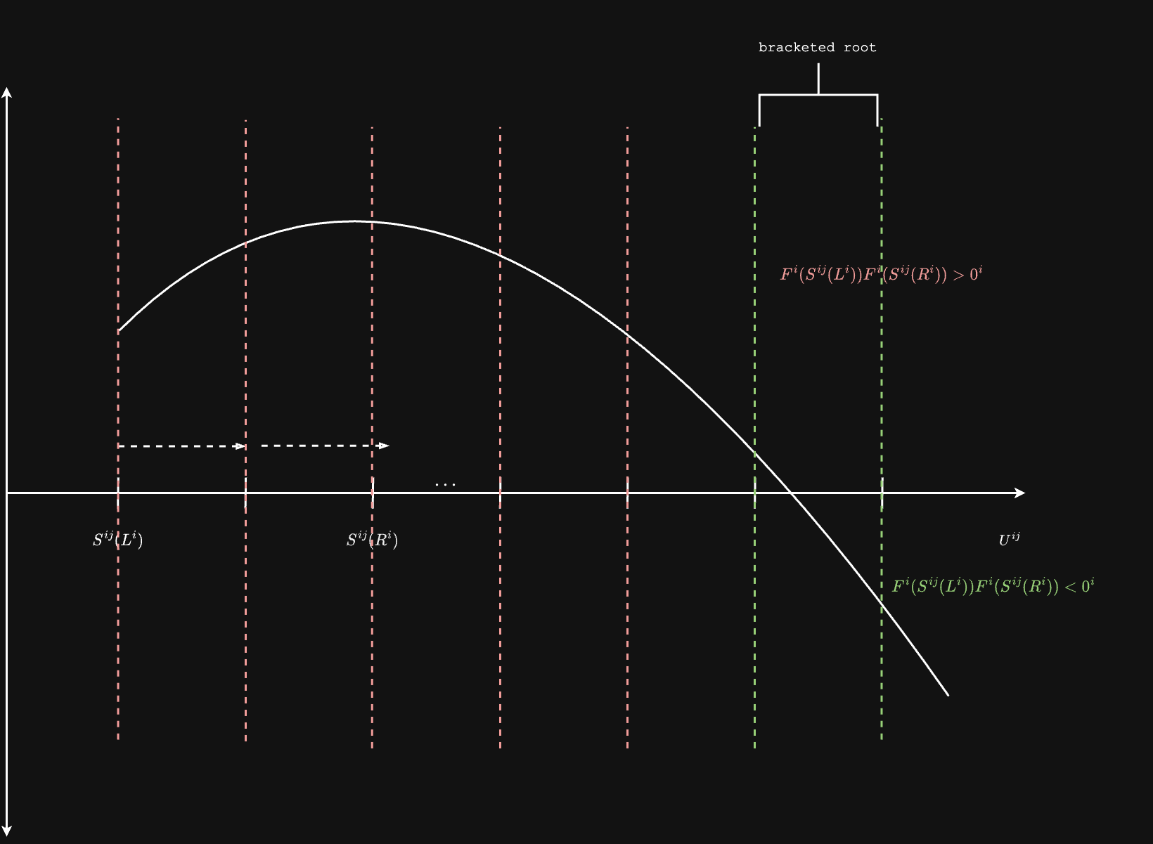
Ray Bracketing Algorithm

The ray bracketing algorithm efficiently finds intervals along rays that contain isosurface intersections. This implementation leverages tensor operations for parallel processing of multiple rays.

Algorithm Steps:

1. Initialize parameters:
   • Tensor field $F^i$, ray origins $X^{ij}$, unit directions $U^{ij}$
   • Step size $\Delta \lambda$, maximum iterations $K_{max}$
2. Initialize ray parameters:
   • $L^i\leftarrow 0$ (left bracket)
   • $R^i\leftarrow L^i$ (right bracket)
3. Iterate until convergence or max iterations:
   • Set $R^i\leftarrow L^i+\Delta \lambda$
   • Evaluate field at right bracket: $F^i(R^i)\leftarrow F^i(S^{ij}(R^i))$
   • Create mask for rays that don't yet have a bracket: $M^i\leftarrow {\mathbb{I}}^i\{F^i(S^{ij}(L^i))\cdot F^i(S^{ij}(R^i))\ge 0^i\}$
   • Update brackets using the mask
4. Return brackets $L^i,R^i$ such that $F^i(S^{ij}(L^i))\cdot F^i(S^{ij}(R^i))<0^i$

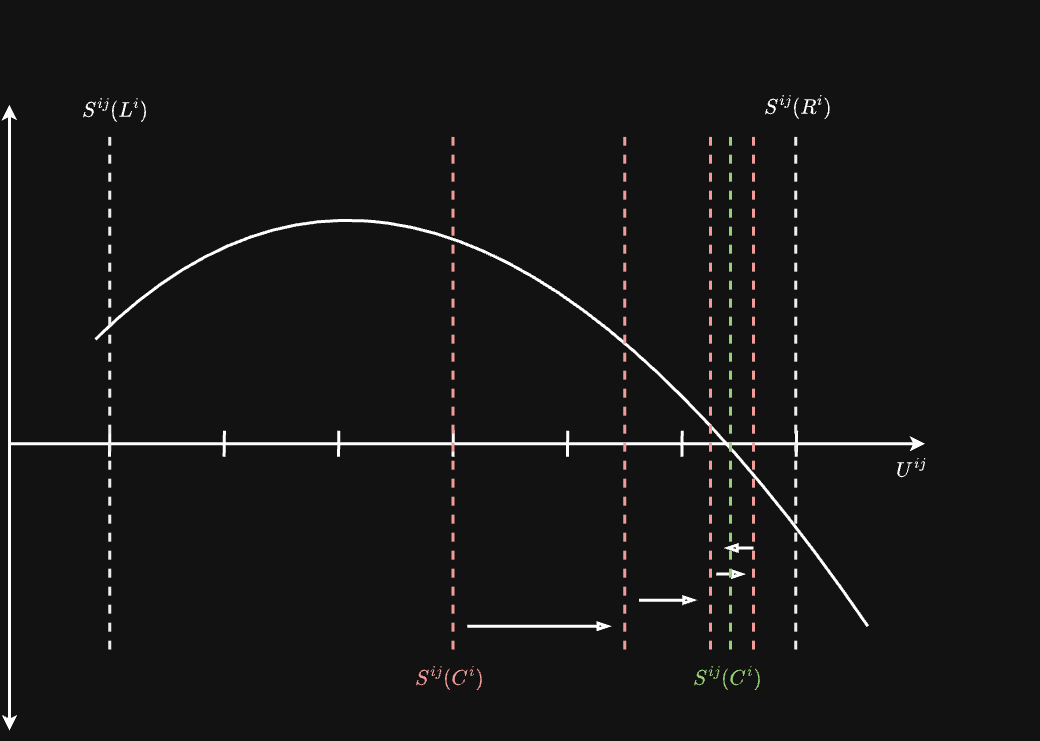
Ray Bisection Algorithm

After bracketing finds intervals containing isosurface intersections, the bisection algorithm refines these brackets to precisely locate the intersection points.

Algorithm Steps:

1. Initialize with bracketing tensors $L^i,R^i$ containing the isosurface
2. Iterate until convergence or max iterations:
   • Compute midpoint: $C^i\leftarrow (L^i+R^i)/2$
   • Create masks for which half contains the root:
     • ${\alpha }^i\leftarrow {\mathbb{I}}^i\{F^i(S^{ij}(L^i))\cdot F^i(S^{ij}(C^i))\ge 0^i\}$
     • ${\beta }^i\leftarrow {\mathbb{I}}^i\{F^i(S^{ij}(R^i))\cdot F^i(S^{ij}(C^i))\ge 0^i\}$
   • Update brackets based on which half contains the root
3. Return refined intersection points

Volume Estimation Methods

This page describes the Monte Carlo volume estimation methods implemented in Crater.rs. Monte Carlo methods were pioneered by Metropolis and Ulam 7 and have become essential tools for numerical computation in high-dimensional spaces.

Consider a scalar field $F^i:{\mathbb{R}}^{n\times m}\to {\mathbb{R}}^m$. We define the region enclosed by the surface as:

$$R^i=\{X^{ij}\in D|F^i(X^{ij})\le 0^i\}$$

Where $D$ is the domain of interest.

Monte Carlo Volume Estimation

Monte Carlo volume estimation is a probabilistic method for approximating the volume of complex regions. This method is particularly useful for high-dimensional spaces where traditional grid-based methods would suffer from the curse of dimensionality.

Algorithm Steps:

1. Generate $N$ random points uniformly distributed in domain $D$: $\{X^{ij}\}\sim \text{Uniform}(D)$
2. Evaluate the scalar field at these points: $V^i=F^i(X^{ij})$
3. Count the number of points inside the region: $C={\sum }_{i=1}^N{\mathbb{I}}^i\{V^i\le 0^i\}$
4. Compute the volume approximation: $V(R^i)\approx V(D)\cdot \frac{C}{N}$

To approximate the volume of $R^i$, we sample $N$ points $X^{ij}\in D$ from a uniform distribution, and count the fraction of points that fall inside the region:

$$\frac{V(R^i)}{V(D)}\approx \frac{{\sum }_{j=1}^N{\mathbb{I}}^i\left(F^i(X^{ij})\le 0^i\right)}{N}$$

Where:

• $V(D)$ is the known volume of the domain $D$
• $V(R^i)$ is the volume we're estimating
• ${\mathbb{I}}^i$ is the indicator function that equals 1 if the condition is true, 0 otherwise

Error Analysis

The error in this approximation decreases as $O(1/\sqrt{N})$, where $N$ is the number of points sampled. This makes it suitable for high-dimensional volume estimation where traditional grid-based methods would suffer from the curse of dimensionality.

The standard error of the volume estimate is approximately:

$${\sigma }_V\approx V(D)\sqrt{\frac{p(1-p)}{N}}$$

Where $p=\frac{V(R^i)}{V(D)}$ is the estimated proportion of the domain occupied by the region.

Alternative Methods

While Monte Carlo methods are the primary approach in Crater.rs, other volume estimation methods include:

• Grid-based methods: Discretize space into regular grids (suffers from curse of dimensionality)
• Analytical methods: Exact solutions for simple primitives (limited applicability)
• Adaptive sampling: Concentrate samples in regions of high curvature or complexity

Monte Carlo methods provide the best balance of generality, accuracy, and performance for complex CSG geometries.

Rescaling Transformations

Rescaling transformations provide mathematically precise control over scalar field output ranges through univariate functions.

Given a scalar field $F^i:{\mathbb{R}}^{m\times n}\to {\mathbb{R}}^m$, a rescaling transformation produces a new field:

$$G^i(\mathbf{x})=\eta (F^i(\mathbf{x}))$$

where $\eta :\mathbb{R}\to \mathbb{R}$ is a univariate function, applied element-wise to the field. This composition preserves the geometric structure of the original field while transforming scalar values according to the chosen function $\eta$.

Function Classes

1. Hyperbolic Tangent Family: Standard and scaled tanh functions
2. Logistic (Sigmoid) Family: Standard and scaled sigmoid functions
3. Arctangent Family: Standard and scaled arctan functions
4. Error Function: Gaussian-like transition with erf approximation
5. Soft Clipping: Linear preservation with asymptotic bounds

Properties of Rescaling

Rescaling transformations maintain several important geometric properties:

1. Isosurface Preservation: If ${\mathcal{S}}_c=\{\mathbf{x}:F^i(\mathbf{x})=c\}$ is an isosurface of $F^i$, then the transformed field has corresponding isosurfaces at $\eta (c)$.
2. Monotonicity: For strictly monotonic $\eta$, the relative ordering of field values is preserved.
3. Bounded Output: Many rescaling functions map $\mathbb{R}$ to bounded intervals, providing guaranteed output ranges.
4. Differentiability: Most rescaling functions are smooth $C^{\infty }$ functions, meaning they have continuous derivatives of all orders. This property is crucial for:
   • Gradient-based optimization
   • Surface normal computation
   • Analytical ray-surface intersection

Rescaling for Ray Cast Stability

Rescaling transformations are crucial for ensuring numerical stability in ray casting operations. Consider the contrived construction:

$f(\lambda )$ is a univariate function, representing the scalar field's value along a single ray. Ray casting is the process of finding a root of $f(\lambda )=0$ to within a tolerance $ϵ$.

The floating point number line is not uniformly distributed. The difference between two adjacent numbers that are representable increases as the numbers get larger. This means for high-gradient fields (e.g., large shapes where, at the isosurface, the field is changing rapidly), there is no representable value of $\lambda$ that can satisfy the tolerance $ϵ$. This is shown in the first inset below.

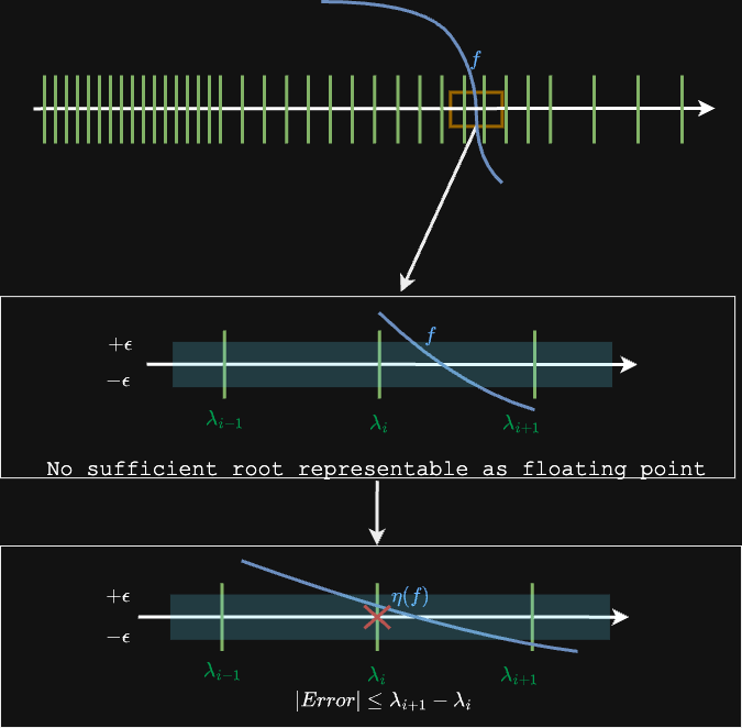
To rectify this, we use our rescaling transformations to map the field values to a closed interval. This has the effect of vertically compressing the field. It is shown in the second inset above.

This method ensures that at least one value of $\lambda$ exists that satisfies the tolerance $ϵ$, and for continuous fields, the converged value of $\lambda$ is at most one floating point number away from the true root.

References

For foundational mathematical techniques:

• Abramowitz & Stegun Handbook of Mathematical Functions (1964) 12
• Press et al. Numerical Recipes (2007) 13
• Boyd & Vandenberghe Convex Optimization (2004) 14

Isosurface Analysis

Surface analysis in crater.rs is based on the properties of scalar fields and their derivatives. Given a scalar field $F^i:{\mathbb{R}}^{m\times n}\to {\mathbb{R}}^m$, we can compute various surface properties.

Gradient Computation

The gradient of a scalar field $F^i$ at origins $X^{ij}$ is the vector of partial derivatives:

$$\nabla F^i(X^{ij})={\partial }^j{F}^i(X^{ij})=\left[\begin{array}{c}{\partial }^j{F}^i(X^{1j})\\ {\partial }^j{F}^i(X^{2j})\\ ⋮\\ {\partial }^j{F}^i(X^{mj})\end{array}\right]$$

In crater.rs, gradients are computed using automatic differentiation through the Burn framework.

Gradient Properties

• The gradient points in the direction of steepest increase of the scalar field
• The magnitude of the gradient indicates the rate of change
• At points on an isosurface $F(x)=c$, the gradient is normal to the surface

Surface Normals

For origins $X^{ij}$ on an isosurface $F^i(X^{ij})=c$, the unit normal vector is:

$$\hat{n}=\frac{\nabla F^i(X^{ij})}{|\nabla F^i(X^{ij})|}$$

Surface Curvature

Surface curvature measures how much the surface deviates from being flat. For a surface defined by $F(x)=c$, the mean curvature is:

$$H=\frac{1}{2}\text{tr}({\nabla }^{2}F)$$

Where ${\nabla }^{2}F$ is the Hessian matrix of second derivatives.

Marching Cubes Algorithm

Marching cubes is one of the most widely used algorithms for isosurface extraction, producing a triangular mesh approximation of the isosurface 1.

In crater.rs, the algorithm is implemented with GPU acceleration using the Burn tensor computation library, making it highly efficient even for large grids.

Overview

The marching cubes algorithm converts implicit surfaces (represented by scalar fields) into explicit triangular meshes. This is essential for visualization, 3D printing, and further geometric processing.

Why Marching Cubes?

• Universal: Works with any scalar field function
• Robust: Handles complex topologies automatically
• Efficient: GPU-accelerated implementation
• Widely Supported: Standard mesh format output (STL, VTK)

Core Algorithm Steps

1. Grid Construction: Create a voxel grid $X_j^i$ with $(n_x+1)\times (n_y+1)\times (n_z+1)$ vertices within a bounding box
2. Field Evaluation: Evaluate the scalar field at each grid vertex: $F^i(X_j^i)$ for all vertices
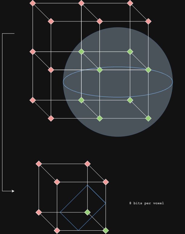
3. Voxel Processing: For each voxel in the grid:
   • Determine which of the 8 corners are inside or outside the isosurface
   • Compute the 8-bit cube index (0-255) based on corner classifications. This can be done with a tensor convolution over $F^i(X_j^i)$ reshaped to $(1,n_x+1,n_y+1,n_z+1)$ with a kernel of shape $(8,1,2,2,2)$ and stride 1.
   • If cube index indicates the isosurface intersects the voxel:
     • Lookup triangle configuration in edge table
     • For each edge intersected by the isosurface:
       • Interpolate vertices to find the exact intersection point
     • Construct triangles using the interpolated intersection points
4. Mesh Assembly: Collect all triangles into a single mesh

Mathematical Foundation

Cube Classification

Each voxel has 8 corners, labeled 0-7. For each corner $k$, we evaluate:

• If $F(corne{r}_k)<0$: corner is inside (bit = 1)
• If $F(corne{r}_k)\ge 0$: corner is outside (bit = 0)

The cube index is computed as: $$\text{index}=\sum _{k=0}^7{\text{bit}}_k\times 2^k$$

This gives 256 possible configurations (0-255).

Edge Interpolation

When the isosurface crosses an edge between vertices $v_1$ and $v_2$ with field values $f_1$ and $f_2$, the intersection point is:

$$p=v_1+t(v_2-v_1)$$

where the interpolation parameter is: $$t=\frac{-f_1}{f_2-f_1}$$

This assumes linear interpolation along the edge.

Interactive Raycast Gallery

Generated automatically via CI/CD using:

cargo run --example raycast-gallery -- --output gallery.html --ray-count 2500

Contributing to Crater.rs

Commit Message Guidelines

Crater.rs uses git-cliff to generate changelogs based on commit messages. Please follow the syntax defined in ./cliff.toml.

Examples

For new features:

feat: new feature added

For bug fixes:

fix: bug squashed!

Development Setup

Building the Documentation

To build and serve the mdBook locally with hot-reload:

./scripts/build-docs.sh --serve

This will start a local server at http://localhost:3000 with automatic reload when you make changes to the documentation.

Running Tests

Before submitting changes, ensure all tests pass:

cargo test

Static Analysis and Styling

Before submitting changes, ensure the project passes lint checks:

./scripts/static-analysis.sh

Release Process (Maintainers Only)

Crater.rs uses cargo-release for automated releases. The release process is handled by CI/CD:

How Releases Work

1. Automated CI/CD Pipeline: The release job in CI configures git for direct push access via OAuth
2. cargo-release Execution: This tool automatically:
   • Runs ./scripts/pre-release.sh which:
     • Executes end-to-end tests and generates artifacts in ./artifacts
     • Runs git-cliff (configured in cliff.toml) to generate changelog
   • Updates version numbers across all relevant files
   • Publishes to crates.io
   • Creates commit with changes tagged as "chore" (skips CI to avoid loops)
   • Adds git tag for the release
   • Pushes changes and tags to the main branch

Creating a Release

As a maintainer, when a merge request lands:

1. The release job becomes available for manual execution
2. Start the job with the appropriate bump level:

   BUMP_LEVEL=(patch|minor|major)
   

Choose the bump level based on the type of changes:

• patch: Bug fixes and small improvements
• minor: New features that maintain backward compatibility
• major: Breaking changes

The automated process handles everything else, ensuring consistent and reliable releases.

Bibliography

Academic Papers

1. Lorensen, W. E., & Cline, H. E. (1987). Marching cubes: A high resolution 3D surface construction algorithm

   • ACM DL • Free PDF
   • Seminal paper introducing the marching cubes algorithm for extracting polygonal meshes from volumetric data.

2. Pasko, A., Adzhiev, V., Sourin, A., & Savchenko, V. (1995). Function representation in geometric modeling: concepts, implementation and applications

   • Springer • ResearchGate PDF
   • Foundational paper for F-rep (Function Representation) modeling, directly relevant to implicit surface work in Crater.rs.

3. Rvachev, V. L. (1982). Theory of R-functions and some applications

   • Wikipedia • Related PDF
   • Theory and applications of R-functions used in CSG operations.

4. Ricci, A. (1973). A constructive geometry for computer graphics

   • DOI
   • Early work on constructive solid geometry for computer graphics.

5. Frisken, S. F., Perry, R. N., Rockwood, A. P., & Jones, T. R. (2000). Adaptively sampled distance fields: a general representation of shape for computer graphics

   • DOI
   • Adaptive distance field representation for efficient shape modeling.

6. Appel, A. (1968). Some techniques for shading machine renderings of solids

   • ACM DL
   • Early work on ray casting and computer graphics rendering.

7. Metropolis, N., & Ulam, S. (1949). The Monte Carlo method

   • JSTOR
   • Introduction to Monte Carlo methods for numerical computation.

8. Hart, J. C. (1996). Sphere tracing: A geometric method for the antialiased rendering of implicit surfaces

   • Springer
   • Sphere tracing algorithm for rendering implicit surfaces.

9. Bloomenthal, J., Bajaj, C., Blinn, J., Cani-Gascuel, M. P., Rockwood, A., Wyvill, B., & Wyvill, G. (1997). Introduction to implicit surfaces

   • Google Books • Amazon
   • Comprehensive introduction to implicit surface modeling and techniques.

10. Requicha, A. A. (1980). Representations for rigid solids: Theory, methods, and systems

    • ACM DL • Semantic Scholar
    • ACM Computing Surveys, 12(4), 437-464 - Foundational work on solid modeling representations.

11. Glassner, A. S. (Ed.). (1989). An introduction to ray tracing

    • Free PDF • Internet Archive • Amazon
    • Morgan Kaufmann - Classic text on ray tracing algorithms and techniques.

12. Abramowitz, M., & Stegun, I. A. (1964). Handbook of Mathematical Functions with Formulas, Graphs, and Mathematical Tables

    • National Bureau of Standards
    • Comprehensive reference for special functions, numerical methods, and mathematical formulas.

13. Press, W. H., Teukolsky, S. A., Vetterling, W. T., & Flannery, B. P. (2007). Numerical Recipes: The Art of Scientific Computing (3rd ed.)

    • Cambridge University Press
    • Practical numerical algorithms and computational techniques.

14. Boyd, S., & Vandenberghe, L. (2004). Convex Optimization

    • Cambridge University Press
    • Mathematical foundations of optimization theory and smooth function analysis.

Software and Libraries

1. Burn Deep Learning Framework

   • Website • GitHub
   • GPU-accelerated tensor computation framework used by Crater.rs.

2. Rust Programming Language

   • Website • Documentation
   • Systems programming language.

3. mdBook

   • Website • GitHub
   • Documentation generator used for this book.